Introduction
2023 started off with lots of buzz about the testing of ChatGPT, the advanced artificial intelligence (AI) chatbot trained by OpenAI to which you can ask questions and get detailed replies across many domains of knowledge. This chatbot has been built over supervised and reinforcement learning (RL) models. We will discuss the latter and the potential of these models in finance.
In October 2022, the Bank of England released the results of a second survey into the state of machine learning in UK Financial Services. Of the firms that took part in the survey, 72% are using or developing machine learning (ML) applications, and according to the article, “firms expect the median number of ML applications to increase by 3.5 times over the next three years.” These applications are becoming more widespread because of the substantial benefits, including increased operational efficiency, enhanced data and analytics, and heightened fraud detection.
Hence, there is interest and the opportunity for new research. We will showcase the application of such tools in finance, and more precisely in portfolio optimization. There is an increasing amount of publications and research on the applications of RL models. For instance, we used the paper, "Asset Allocation: From Markowitz to Deep Reinforcement Learning," published by Ricard Durall, as a reference and for the code. In his publication, he studies OpenAI’s models and shows how some surpassed traditional portfolio optimization techniques. One of these models, called Proximal Policy Optimization (PPO), was selected (for this study), and a series of tests were run using the S&P/IPSA as benchmarks, where six stocks were selected and assigned weights defined by the model. This is our first opportunity for further research, extending our study to the rest of the models and to evaluate performance.
Proximal Policy Optimization Model
The RL model’s goal is to maximize reward. The reward is an indicative parameter for training purposes, and the model achieves this through the interaction of two main components: the agent and the environment. The agent decides which actions to take inside the environment, and such decisions are governed by a policy.
The policy (π, which is based on a state of the environment is updated or enhanced during the training period. Hence, the challenge is the size of the policy update. The PPO model uses a method that guarantees that the new changes in policy are restricted to a range rather than adding penalties or adding optimization constraints, and it does this through a simplified algorithm, compared with similar RL models. The PPO model updates the policy by maximizing:
Where:
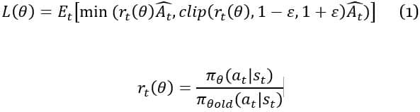
Equation 1 shows how the probability ratio rt is clipped at 1-ε or 1+ε depending on whether the advantage Ât (the quantity that describes how well the action is compared to the average of all actions) is positive or negative. This removes the incentive for moving rt outside the region [1-ε, 1+ε], discouraging overly large updates. Essentially, if the updated policy deviates from the old policy by more than ε, the new policy does not move far away from the old policy.
The optimization of equation 1 and derivation of losses can be computed with minor changes to a typical policy gradient implementation and by performing multiple steps of stochastic gradient ascent on this:
Where:

Methodology
The project was divided into two main parts: stock selection and definition of stock’s weight. For stock selection, we used the “cluster” methodology, where six clusters were defined for those stocks inside the benchmark with enough price history (at least 70% of prices available in a ten-year sample). Once the clusters were defined, the stock with the highest return adjusted by risk was selected inside every cluster. There were some clusters with only one stock, as seen in Figure 1.

The covariance matrix and mean return between January 2010 and December 2019 were used to define the clusters, and the number of clusters was decided by reviewing the silhouette coefficient (silhouette coefficient or score is a metric used to calculate the performance of a clustering technique) and charts. This could be a second opportunity for further research on the methodology and implementation to enhance results. For instance, we could fine-tune the inputs and use this for every portfolio rebalance to pick the stocks. In our current study, we ran this only once and the portfolio remained with the same stocks for the rest of the study.
The portfolio framework calculated values on a daily basis, considering holidays, rebalance, and costs. Two versions of the portfolio were calculated: gross and net return. The former is the result of price return only, and no dividends were included, while the latter is the gross return minus the run cost and rebalance cost. Run cost is an annual amount of 1%, while the rebalance cost is 1% for the whole amount of units bought and sold in every rebalance. These are just reference numbers but could be adjusted as desired.
Calculations
With the current list of constituents in the benchmark, prices were downloaded from Yahoo Finance's API between January 2010 and December 2022, removing those stocks missing more than 30% of prices. Hence 25 out of 30 stock passed such filter.
Holidays were used to generate a list of business days and rebalance dates. In our study, rebalance had been set on a quarterly basis. However, this could be a third opportunity for further review, where we could modify time frames such as monthly, semi-annually, etc.
The stocks selection was performed through a "cluster" methodology, and the following six stocks were selected: ['CMPC.SN','IAM.SN','VAPORES.SN','CAP.SN','ORO-BLANCO.SN','CHILE.SN'].
Data before January 2018 was used to train the model and calculate weights for the inception of the portfolio. Every quarter rebalance triggered the model training after adding the past three months of stock prices, meaning the model was trained again from 2010 to the current date, capturing the latest market information.
The following inputs and models were evaluated:
- PPO model using current price as the input for the following two versions:
- Model training, reset, and inquiry weights
- Model training and inquiry weights
- PPO model using covariance matrix of price returns for the last 252 business days
- Mean-variance portfolio optimization (the traditional approach and used as a reference along with S&P/IPSA price and total return)
Before looking into the results, is important to highlight the reward, one of the main parameters used by RL models to reach the optimum. In this study, the reward is calculated after every step during the training period and is the result of difference between the end total portfolio value (after new positions have been taken) and the beginning total portfolio value (before new position). Figure 2 shows how the model starts losing money, but right after 15,000 training iterations, it starts to gain and remains as such for the rest of the training period.

It is typical for PPO to perform many timestep updates on a batch of training data using mini-batch gradient descent (picking out a small number of randomly chosen training inputs). Data is reused through tens of training timesteps and many mini-batch per timesteps. Based on this and performance achieved by the reward in Figure 2, it appears that the data is enough to use in the PPO model.
After comparing all of the results, the best performance came from the PPO B model, using prices as the input and estimating weights right after training. Table 1 shows a summary of metrics for the period between January 2018 and December 2022:
|
Model
|
Annualized Return
|
Annualized Volatility
|
Return Adj by Risk
|
|||||||||
|---|---|---|---|---|---|---|---|---|---|---|---|---|
|
PPO (A) Prices with reset
|
2.47%
|
26.8%
|
0.0921
|
|||||||||
|
PPO (B) Prices without reset
|
17.6%
|
29.01%
|
0.6066
|
|||||||||
|
Mean-Variance
|
4.6%
|
24.3%
|
0.1892
|
|||||||||
|
S&P IPSA Index (CLP) TR
|
-1.37%
|
22.95%
|
-0.0597
|
|||||||||
Table 1
Figure 2 shows the comparison between the benchmark price and total return and the PPO A model. Returns are RLG_IL (gross) and RLN_IL (net).
The portfolio with the PPO model using the covariance matrix for the past year as the input (RLGCOV_IL and RLNCOV_IL) performed better than the PPO model A and mean-variance. However, the PPO B model beat them all.
Figure 3 shows the portfolio values of the PPO B model, or the enhanced PPO model (i.e., model training and estimating weights right away). The difference between PPO A and PPO B used in Figures 2 and 3 is the timing when weights are calculated. Both are generated after model training, but only the latter weights are generated right after the model has been trained. There is no reset. Enhanced values are RLP2G_IL (gross) and RLP2N_IL (net).


Conclusion
The RL PPO model performed better than the traditional optimization methodology and the benchmark. In this case, the returns over five years using the PPO B model for asset allocation was 17.6%, while the benchmark was -1.3%. Adjusting for risk, the former had a value of 0.6, while the latter had less than zero. However, this is just a first test and would require further study and testing with distinct scenarios and markets, as well as valuation of more methodologies. There is a significant difference on how RL models are set up and used despite inputs, and using weights right after model was trained (i.e., training sample includes rebalance date) yielded the best results.
References
Ricard Durall. "Asset Allocation: From Markowitz to Deep Reinforcement Learning." Open University of Catalonia.
Gaurav Chakravorty, Ankit Awasthi and Brandon Da Silva. "Deep Learning for global tactical assets allocation"
Markus Holzleitner, Lukas Gruber, Jose Arjona-Medina, Johannes Brandstetter and Sepp Hochreiter. "Convergence Proof for Actor-Critic Methods Applied to PPO and RUDDER." Johannes Kepler University Linz, Austria.
John Schulman, Philip Moritz, Sergey Levine. Michale I. Jordan and Pieter Abbel. "High-Dimensional Continuous Control Using Generalized Advantage Estimation." University of California Berkeley.
Talk to One of Our Experts
Get in touch today to find out about how Evalueserve can help you improve your processes, making you better, faster and more efficient.


