Have you ever wondered why we are so captivated by the power of forecasting? It's not just a matter of curiosity, it's also a vital tool for making informed decisions and acting based on what could lie ahead. Whether it's predicting the weather, prices, elections, or any other aspect of our lives, having a glimpse into the future could mean the difference between success and failure.
In terms of pricing, especially stock pricing, there are many publications and papers discussing the strengths of distinct valuation methodologies, such as linear and nonlinear modeling. For instance, over the past 20 years, interest in artificial neural networks (ANNs) for nonlinear modeling suggests it could be an alternative for traditional forecasting methods like the Autoregressive Integrated Moving Average (ARIMA) model, which is a popular linear model that has been challenged by the performance of ANNs. There are also studies similar to those conducted by professor G. Peter Zhang suggesting the usage of both when performing forecasts with time series. We intend to add insights to this debate with our study, highlighting applications to the Chilean market.
In our previous blog called “Reinforcement Learning Models and Asset Allocation,” we introduced a case for the usage of Reinforcement Learning (RL) models to construct a portfolio using the S&P IPSA Index as a benchmark. We concluded that the RL model (Proximal Policy Optimization [PPO]) used to run the study was successful against the mean-variance portfolio and benchmark. Hence, the next question would be if the PPO model could beat a known ARIMA model when forecasting stock prices and the best expected performers. We believe this is a valid question, not just because of the debate mentioned above, but also to test such models in developing countries.
Data
The data extracted were the closing prices of the S&P IPSA’s current stocks. The source was Yahoo Finance, and the pricing period ranged from 1 January 2012 to 1 January 2023. We used only the stocks with more than 70% of available pricing over the timeframe, narrowing it down a total of 25 stocks to select from each rebalance.
Using the Chilean market holidays, portfolio business days were generated. Portfolio valuation ranged from 2 January 2018 to 28 December 2022.
Methodology
We used a statistical analysis model called Autoregressive Integrated Moving Average (ARIMA) to forecast forward three-month stock prices. Some important usage facts of this model are as follows:
- Past values (Autoregressive AR) over the variable of interest are defined as (p)
- Differences between the current values and the previous values (removing any trends or seasonal structures) are defined as (d)
- Dependency between observation and residual error (Moving Average [MA], which captures the influence of noise or outliers) is defined as (q)
- Hence, the model setup for a particular time series is: ARIMA (p,d,q)
Before working with the ARIMA model, stock prices were analyzed and tested using Dickey-Fuller ADF, KPSS, and Phillips-Perron to define the correct amount of differencing. After this, using the auto_arima function, which is a pmdarima tool (Python module), the number of lags were defined for every stock based on the Akaike Information Criterion (AIC).
The inception date of the portfolio was 2 January 2018, and all previous years were used to setup and train the model. However, the portfolio rebalances quarterly. Hence, every time the portfolio was rebalanced, the model was trained again and asked to forecast the next three months.
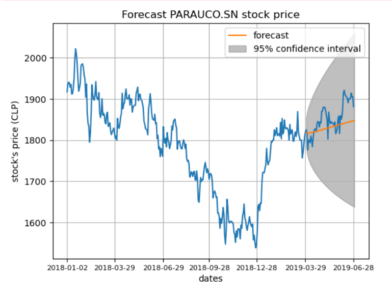
Example. Stock: PARAUCO.SN, forecast date: 29 June 2018
We used the closing prices of PARAUCO.SN from 1 January 2012 to 29 March 2018 and ran auto_arima to find the best possible model within the order constraints provided according to AIC; the selected model was: ARIMA (1,1,1).
- p=1, the number of lag observations or autoregressive terms in the model
- d=1, the difference in the observations
- q=1, the size of the moving average window
The p-value of AR(p) and MA(q) coefficients were 0.000, meaning that p and q are statistically significative in the model.
|
|
coef
|
std err
|
z
|
P>|z|
|
|---|---|---|---|---|
|
intercept
|
0.2030
|
0.133
|
1.531
|
0.126
|
|
ar.L1
|
0.6230
|
0.083
|
7.478
|
0.000
|
|
ma.L1
|
-0.7232
|
0.074
|
-9.813
|
0.000
|
|
sigma2
|
325.9698
|
7.244
|
45.001
|
0.000
|
The model was used to predict the closing price as of 29 June 2018. Figure 1 shows the historical price and the forecast for the following three months.
The model was used to predict the closing price as of 29 June 2018. Figure 1 shows the historical price and the forecast for the following three months.

Where:
Wi,t = weight of stock i on rebalance as of t
ranki,t = rank of stock i on rebalance as of t
When there were less than six stocks with a positive expected return, the rest of the weight was allocated to cash and accrued with an annual interest of 0.5% until the next rebalance.
Results
Figure 2 highlights the portfolio levels in gross (ILF_G) and net (ILF_N) pricing, 1% cost for both: run and rebalance cost) between January 2018 and December 2022 versus the benchmark (S&P IPSA), which has been rebased for comparison purposes. As shown, the COVID crisis did have an impact on the strategy. However, the index has recovered faster than benchmark. Moreover, the forecast strategy generated a 0.42 risk-adjusted return for the entire period, while the benchmark was less than zero.

Figure 3 can help us answer or provide some insight on which model, either RL or ARIMA, has better performance (higher returns) in the Chilean market. It is important to acknowledge that this is just a sample between January 2018 and December 2022, and although it includes the pandemic, further studies are recommended.

The new terminology, MVG_IL and MVN_IL, refers to the gross and net mean-variance portfolio, while RLP2G_IL and RLP2N_IL refer to the gross and net for the RL portfolio. While the gross RL portfolio had an annualized risk-adjusted return of 0.6, the ARIMA gross portfolio was 0.42 for the entire period. However, it is worth noting the outperformance shown by the latter before COVID, suggesting that a mix of strategies could yield even better performance for the investor.
Conclusion
Exciting findings from this study reveal the immense value in employing forecast methodologies to handpick stocks and construct portfolios based on projected positive performance. The approach involved selecting the top six stocks with the highest anticipated positive performance and allocating them accordingly, resulting in a decreasing allocation strategy. When there was less than six stocks with a positive performance outlook, we strategically allocated to cash until our next rebalance date. The research has uncovered a powerful tool that can help investors make informed decisions and achieve better returns than the benchmark.
Also, when comparing the results between traditional approaches like the mean-variance portfolio, ARIMA forecasting portfolio, and RL portfolio, we find RL outperforms with an annualized risk-adjusted return that is 0.18 higher than ARIMA’s for the sample period. However, the fact that ARIMA outperformed before COVID suggests the coexistence of linear and nonlinear patterns inside the market. For this reason, further studies where both methodologies are used for selection and allocation are encouraged to uncover more insights about Chilean market and portfolio construction.
Talk to One of Our Experts
Get in touch today to find out about how Evalueserve can help you improve your processes, making you better, faster and more efficient.


